Live on Forge: 30 Minute Hyperliquid Liquidity Outlook

Introducing the 30-minute Hyperliquid Liquidity Outlook, a new topic on the Allora testnet for predicting displayed order-book depth across 20 markets.

The topic predicts average depth within defined price bands around the midprice during minutes 15–30 after each round opens. It measures the liquidity visible in the top 20 price levels on each side of the book.

This is Allora’s first topic focused on order-book depth. Below, we’ll explain the prediction objective, its relevance to trade execution, and how to build a model for the topic.

Prediction Objective

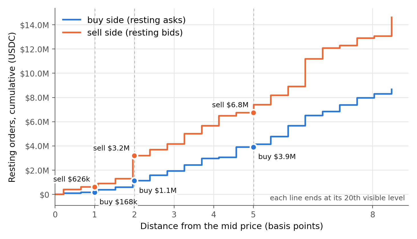
The Liquidity Outlook predicts average displayed order-book depth within 1, 2 and 5 basis points of the midprice, separately for bids and asks. The midprice is halfway between the best bid and the best ask; one basis point is 0.01% of the price.

Depth is measured as the total quote notional of orders inside each band: price multiplied by quantity, summed across the included levels. For the USDC-quoted markets described here, depth is expressed in USDC.

Only the top 20 price levels on each side are counted. The target is therefore captured depth, which may exclude orders further into the book even when they fall within the specified band. The bands are cumulative: depth within 5 basis points includes depth within 1 and 2 basis points.

In the illustrated ETH book, the captured asks within 5 basis points total 150,000 USDC, and the captured bids within 5 basis points total 180,000 USDC. The asks represent liquidity available to buyers; the bids represent liquidity available to sellers.

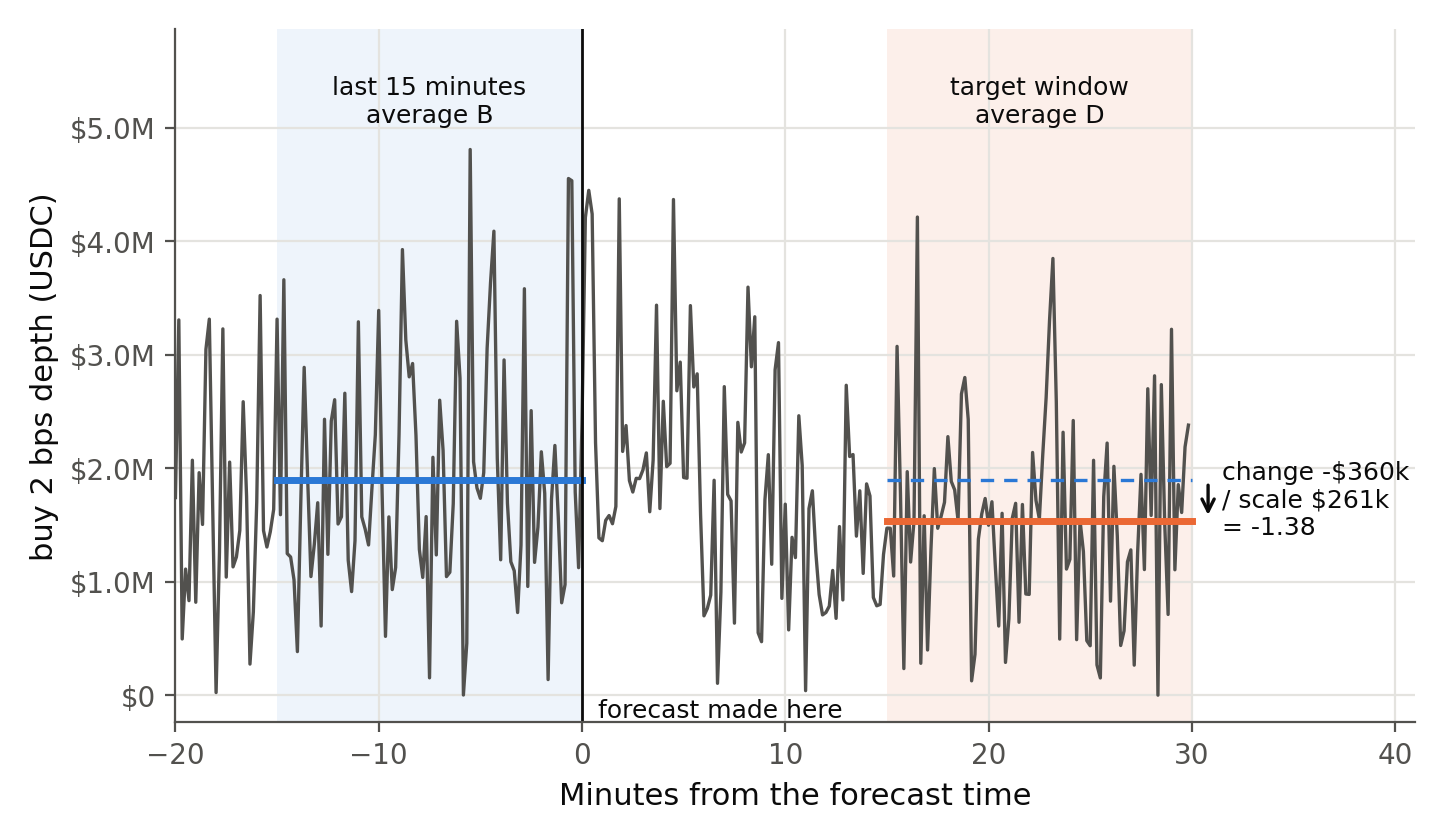
The topic predicts average captured depth during minutes 15–30 after each round opens. Each depth measurement uses the midprice at that time. A round opening at 12:00 therefore targets average depth from 12:15 to 12:30.

For each market, side and band, the inference is defined as:

y = (D − B) / S

where:

The research specification proposes defining S as the root-mean-square change between future and trailing average depth over the calibration sample, with a minimum of one quote-currency unit:

S = max( 1, √( (1/K) × Σ(k = 1 .. K) (Dₖ − Bₖ)² ) )

Here, K is the number of calibration observations. The calibration period and resulting scales are published with the topic configuration.

For example, if the trailing average is 200,000 USDC, the scale is 100,000 USDC, and predicted future average depth is 150,000 USDC, the inference is −0.5. An inference of zero represents no change from the trailing average; positive values indicate greater depth and negative values indicate less depth.

The ground-truth value uses the same definition, replacing predicted depth with realized depth:

y = (D − B) / S

Three bands on each side produce six inference values per market, or 120 across the 20 markets.

The topic covers 20 markets: ten crypto perpetual markets on Hyperliquid—BTC, ETH, SOL, XRP, HYPE, DOGE, ZEC, TRX, BNB and NEAR—and ten markets on trade.xyz covering gold, WTI crude oil, Brent crude oil, silver, natural gas, copper and four stock index products.

Why it Matters

For a trader planning an order, the relevant question is how much liquidity will be available when they execute. Less depth near the midprice means an order of a given size may consume liquidity further into the book, increasing slippage.

The Liquidity Outlook provides an estimate of whether that depth will increase or decrease relative to its recent average. A trader planning to buy could use the ask-side estimates when deciding when to execute or how to divide an order into smaller trades. Someone reducing a position could use the corresponding estimates for the side they need to trade against.

The intended benefit is better execution planning. Whether these inferences actually reduce trading costs requires a separate evaluation; the model example below tests prediction accuracy.

Worked Example

We wanted to test whether a model using only the last 15 minutes of order-book data could outperform a no-change baseline on unseen rounds. That baseline always returns an inference of zero: future average depth is expected to equal the trailing 15-minute average. We put together a Python walkthrough and a small collector to test this.

The collector reads each market’s book from Hyperliquid’s public info endpoint every 10 seconds and stores the observations locally. The endpoint provides the current book, so building a training dataset requires collecting a history.

A failed or invalid read is recorded as missing data, not zero liquidity. A valid two-sided book can still have no orders within a particular band; in that case, the measured depth is genuinely zero.

The example fits the models using 90 minutes of books from 28 October plus the first hour of a three-hour collection on 3 November, then tests them on the remaining data.

For each snapshot, the midpoint is calculated from the best bid and best ask. Using up to 20 price levels per side, the collector measures depth within 1, 2 and 5 basis points of that midpoint. Ask-side depth measures liquidity available to buyers; bid-side depth measures liquidity available to sellers. Each value is the total USDC notional of the orders inside its band:

depth = Σ price × size, over the levels inside the band

If a side has 20 visible price levels and the twentieth lies strictly inside the band, the example marks that measurement as capped. The depth is still the sum of the captured orders within the band, but the feed cannot establish whether additional orders lie beyond those 20 levels.

For each round, the example calculates B from the 15 minutes before the round opens and D from minutes 15–30 afterward. A round opening at 12:00 therefore uses a baseline window of 11:45–12:00 and a target window of 12:15–12:30. Each window contains 90 sampling points, spaced 10 seconds apart.

The example accepts a window when at least 80 of its 90 readings are valid and averages those valid readings. This differs from the research specification’s stricter requirement that all 90 points be valid, so the example is not an exact reproduction of that ground-truth contract.

The example estimates a separate scale for each market, side and band using only the fitting data:

S = √( average of (D − B)² ), and at least 1 USDC

For live submissions, the worker must use the topic’s published baseline and fixed scales rather than the scales estimated for this example.

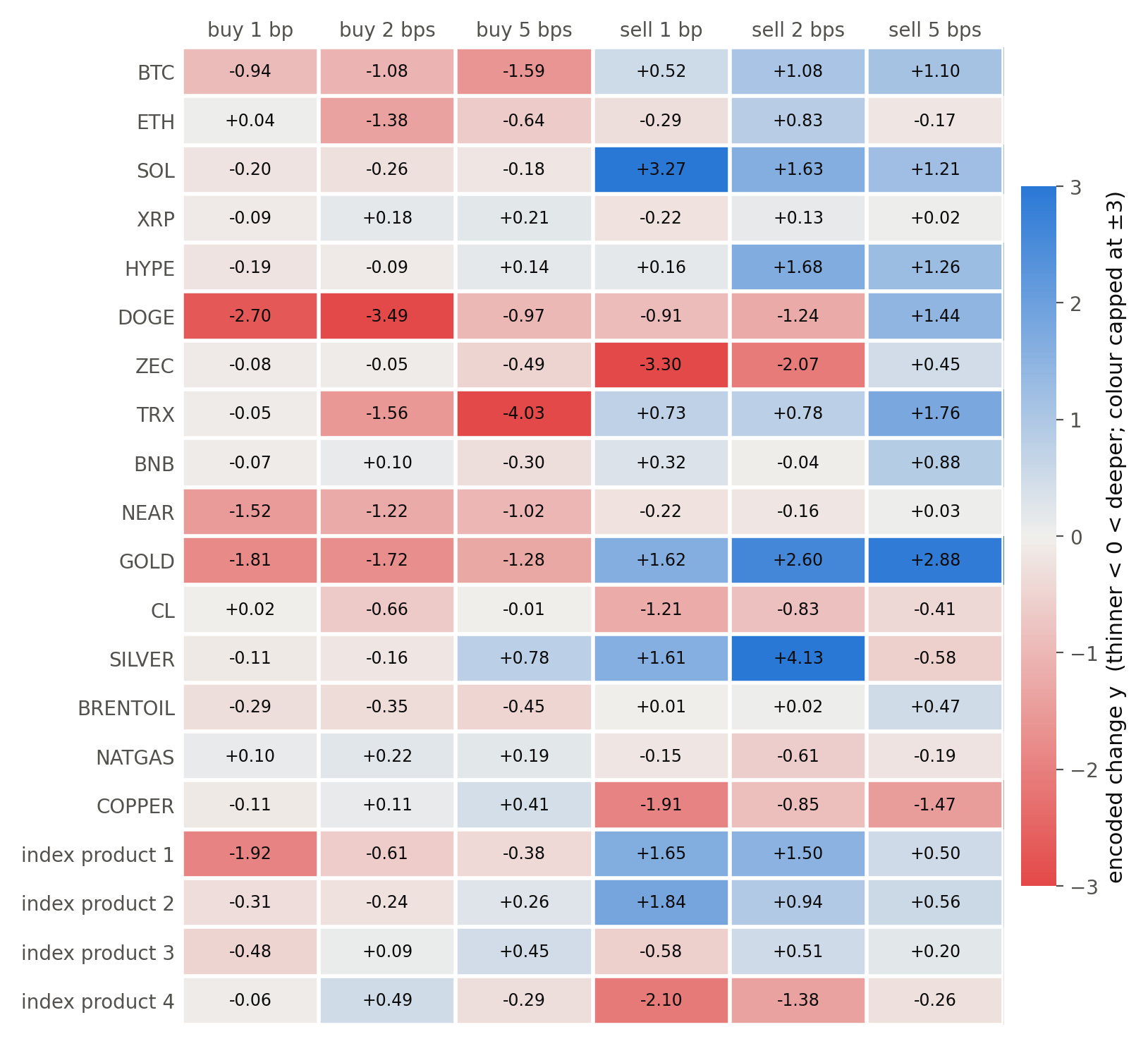
The first model is the zero-change baseline. The second, called “carry,” uses the difference between the latest depth reading, N, and the trailing 15-minute average, B, to predict the future change:

ŷ = β × clip( (N − B) / S, ±5 )

A separate coefficient β is fitted for each band and side using least squares across all 20 markets. Clipping the normalized input to between −5 and +5 limits the influence of extreme readings. A third model also uses M, the average depth over the last 5 minutes:

ŷ = β₁ × clip( (N − B) / S, ±5 ) + β₂ × clip( (M − B) / S, ±5 )

The models are fitted on data before a chronological cutoff and tested on rounds afterward. A 45-minute gap separates the fitting and test periods to prevent overlap between their feature and target windows.

For evaluation, squared error is calculated for each inference, averaged across each market’s six values, then equally across markets, and finally across test rounds. This is the example’s loss. For the zero-change baseline, the loss is simply the average of y². Improvement relative to that baseline is measured as:

error saved = 1 − loss(model) / loss(zero)

A positive value indicates lower loss than the zero-change baseline; a negative value indicates higher loss. The example also reports directional accuracy: how often the model correctly predicts whether average depth increases or decreases relative to the baseline.

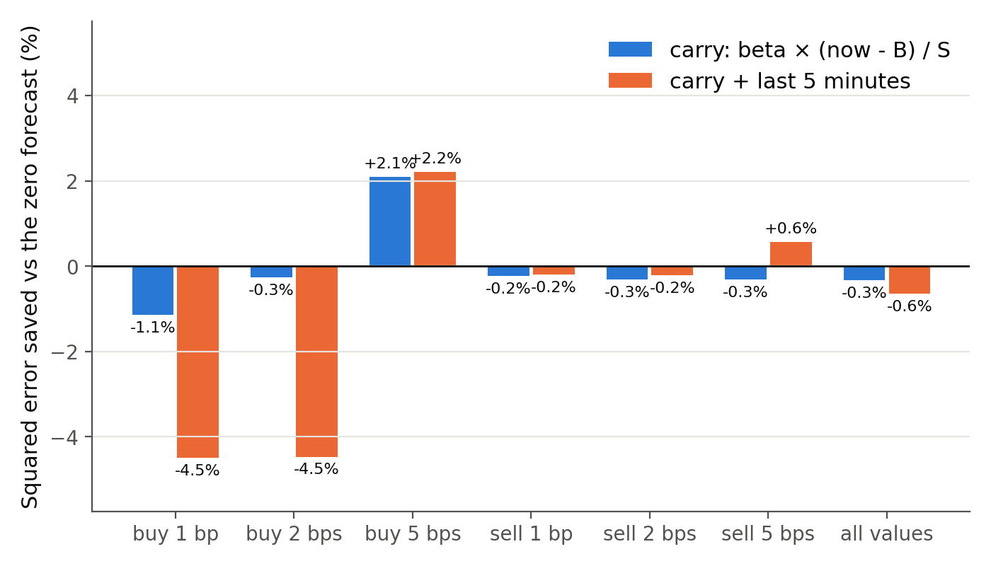
Across the six held-out rounds, the carry model’s squared-error loss was 0.3% higher than the zero-change baseline, with directional accuracy of 54%. It therefore did not improve on the baseline overall.

It did reduce loss on 13 of the 20 markets, with the largest improvements on BTC and ETH. These gains were outweighed by errors elsewhere. ZEC accounted for most of the baseline’s loss because its depth changes were large relative to its estimated scales. This illustrates how strongly scale calibration can affect the aggregate result.

With only six test rounds from a few hours of data, these results are a preliminary check of the method. A longer evaluation across different sessions and market conditions is needed to assess predictive performance.

The worker maintains a rolling 15-minute history of order-book observations and returns a dictionary mapping topic labels to inference values, such as hl/eth/buy/depth01bps. Inputs must be available by the round’s opening timestamp; the submission window does not extend that information cutoff. Live submissions must use the topic’s shared baseline and fixed scales.

The example follows the worker structure used in the Forge Builder Kit and refuses to run until a topic ID is configured:

TOPIC_ID = None  # set to 91 to target the testnet topic

def __call__(self, context):
    # last 15 minutes of books -> six values per market -> clip((N - B) / S, 5) -> times beta
    return {"hl/eth/buy/depth01bps": 0.12, ...}

What makes this topic challenging

Resting orders can be cancelled at any moment, so displayed depth can change rapidly. A window average can also conceal brief periods of thin liquidity. Predicting that average does not guarantee the liquidity available when a particular order arrives or the price at which it will execute.

For the trade.xyz markets, session timing is another potential source of variation. These perpetuals trade around the clock, while their underlying markets have defined trading hours. Models may need to account for differences between those sessions.

The 20-level capture limit also affects what the topic measures. In the 28 October BTC sample, the visible levels extended only about 2–3 basis points from the midprice. The 5-basis-point measurement therefore represented the entire captured side of the book, potentially excluding additional orders within that band. The captured value can still increase or decrease, but it does not necessarily represent complete depth within 5 basis points.

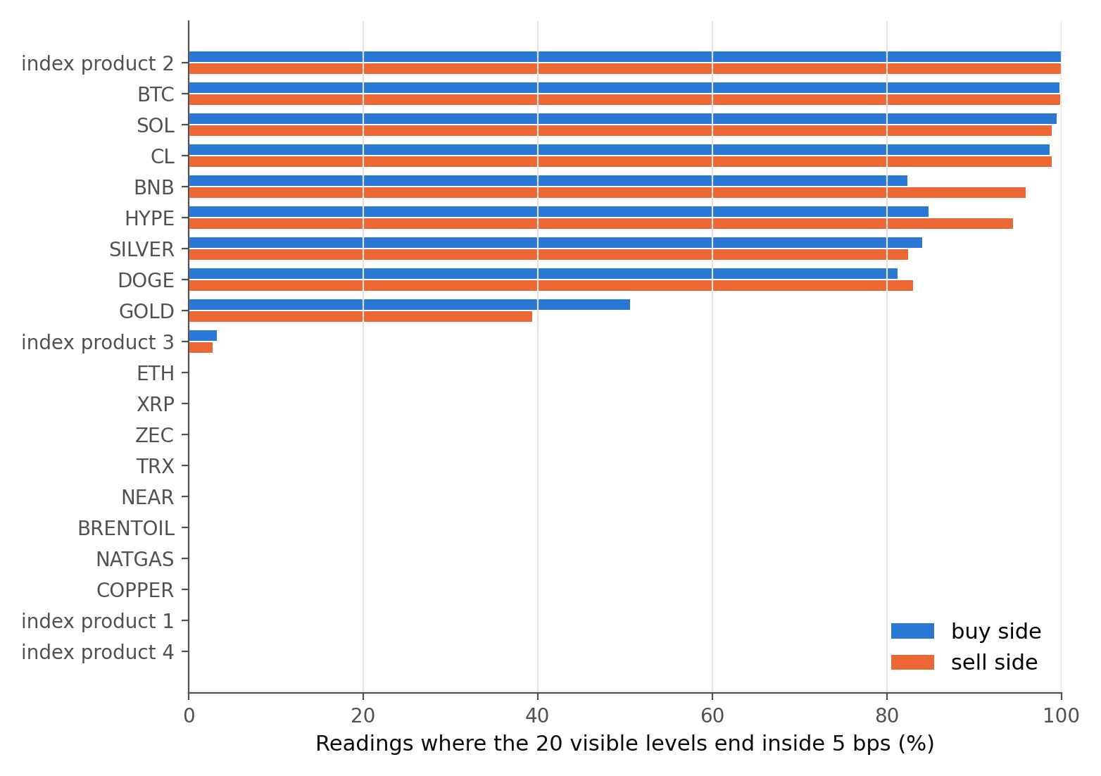
A few open questions I expect testnet to answer, so that means you guys:

Build against it

If you already build short-horizon models using Hyperliquid data, this walkthrough provides a starting point for modelling captured order-book depth. Use the topic’s target windows, normalization and fixed label schema when adapting your own model.

Once the walkthrough is published, download the code and collect an initial dataset. Run the example unchanged first to check the pipeline and inspect its results on held-out rounds. A few hours of data are enough to try the workflow; evaluating predictive performance requires a longer history.

Start Building Your Model on Forge

‍