Allora recently introduced triple-barrier topics for Gold, Silver, and Oil on Forge testnet. The new Builder Kit walkthrough takes the next step: an example you can run, inspect, modify, and deploy as a worker submitting probabilities to the network.
The example follows the entire modeling process, from historical candles and target construction to model selection, held-out evaluation, and live inference. Along the way, it shows how a three-class prediction problem connects to a simple trading decision.
We use Gold throughout this walkthrough. The same script supports Silver and WTI oil:
| Asset | Testnet topic | Atlas dataset |
|---|---|---|
| Gold | 87 | hl_xyzgold_1min |
| Silver | 88 | hl_xyzsilver_1min |
| WTI oil | 89 | hl_xyzcl_1min |
The example uses real one-minute OHLCV history for these Hyperliquid markets, collected and served through Atlas, Allora’s data platform. The Builder Kit already includes an Atlas data adapter: setting data_source="allora" in AlloraMLWorkflow selects it, and tickers=["hl_xyzgold_1min"] selects Gold. The workflow fetches and caches the available historical candles for training; the deployed model uses the same adapter to fetch fresh market data for live predictions.
What are we predicting?
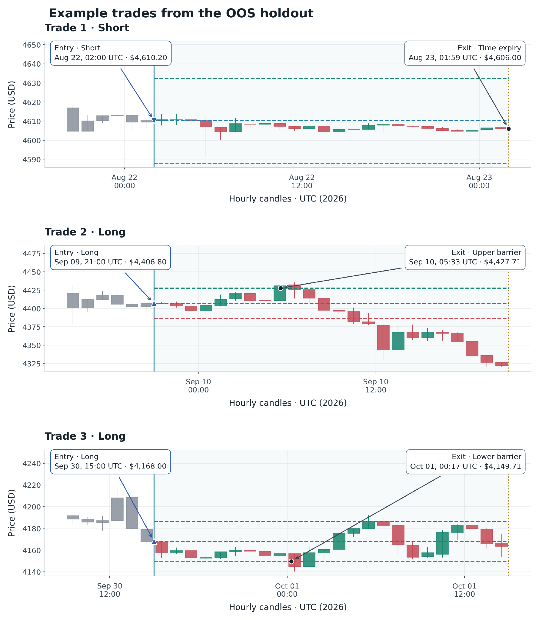
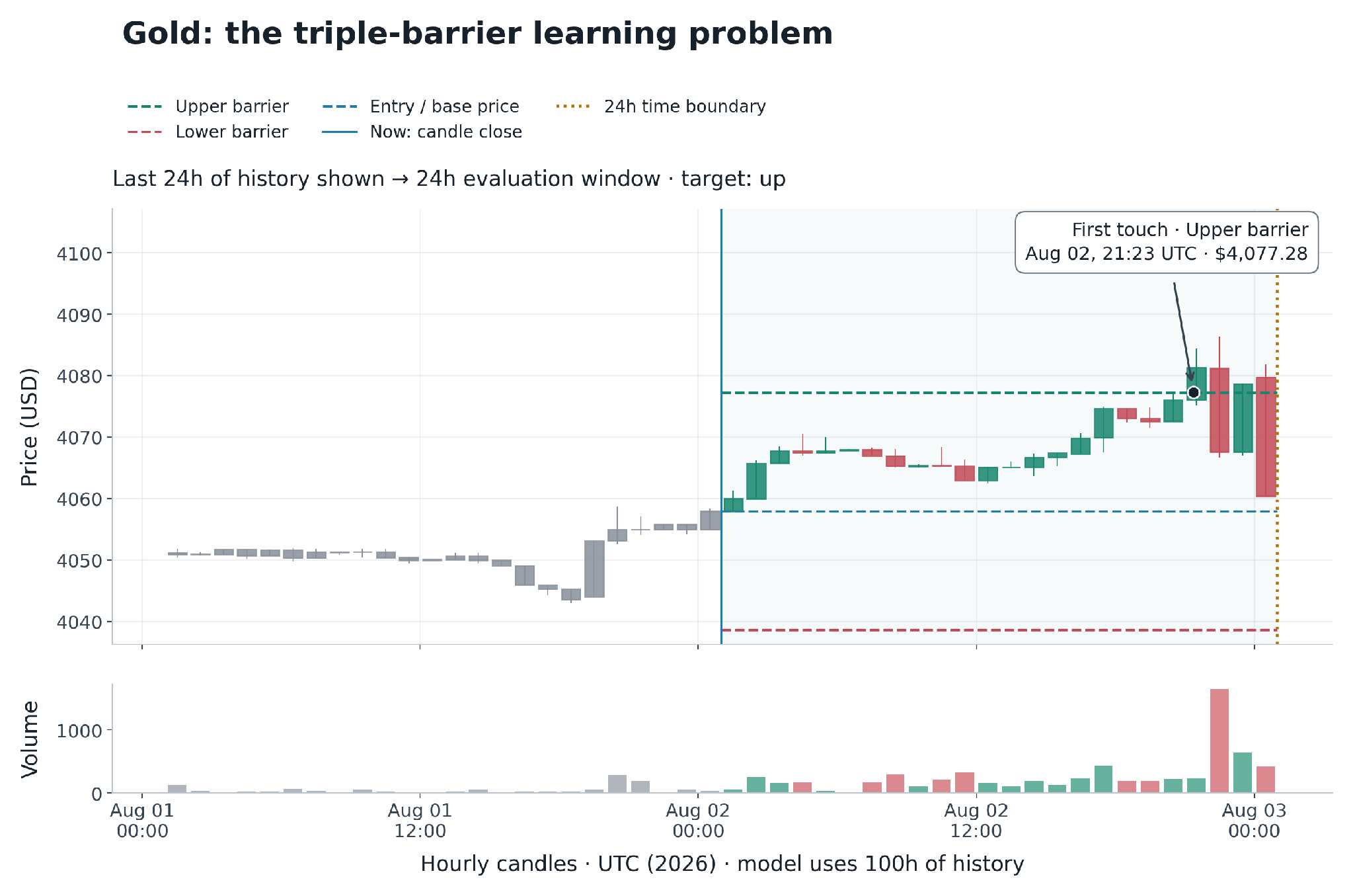
At each prediction time, draw an upper and a lower price barrier from the last observed transaction price, and a time boundary 24 hours ahead. The target is determined by which price barrier the market touches first. If neither is touched before expiration, the target is neutral.

The example resamples Atlas minute data into hourly bars. Each row's timestamp is the opening time of its candle, so the prediction time is that timestamp plus one hour. At that point, the model can observe that completed candle and all preceding candles. We give it the most recent 100 hourly bars as normalized OHLCV features.
Barrier width adapts to historical price movement. The volatility estimate averages rolling high–low log ranges over 100 target horizons: 2,400 hours for these 24-hour topics. With this average called ATR, the boundaries are:
base = close of the minute candle opening at T − 1 minute
upper = base × exp(0.25 × ATR)
lower = base × exp(−0.25 × ATR)
Here, ATR means an average rolling high–low log range, rather than conventional average true range. The reputer selects hourly openings in [T − 2401h, T − 1h), then computes each range over the inclusive window [t − 24h, t] within that selection.
The model uses hourly features, but labels are checked against minute highs and lows. Starting with the candle opening at T − 1m, inspect candles through the half-open interval ending at T + 24h − 1m:
- Down: the lower barrier is touched first.
- Up: the upper barrier is touched first.
- Neutral: neither barrier is touched before expiration.
If both barriers are touched in the same minute, down wins the tie. Missing required candles leave the target unresolved. The triple-barrier documentation is the reference for these exact conventions and evaluation rules.
A familiar classification problem
Once those labels are attached to the historical rows, this is a three-class classification problem. Most off-the-shelf classifiers can tackle it, especially estimators with the familiar scikit-learn fit and predict_proba interface.
The example uses LGBMClassifier. Targets are stored as one-hot columns—target_down, target_neutral, and target_up—and converted to class indices for fitting. Predicted probabilities are stored in matching pred_ columns. A worker submits the full labeled distribution, for example:
{"down": 0.2, "neutral": 0.3, "up": 0.5}
The highest-probability class is useful for accuracy, confusion matrices, and the trading illustration below. The network receives all three probabilities, preserving the model's uncertainty.
Train on the past, evaluate on what comes next
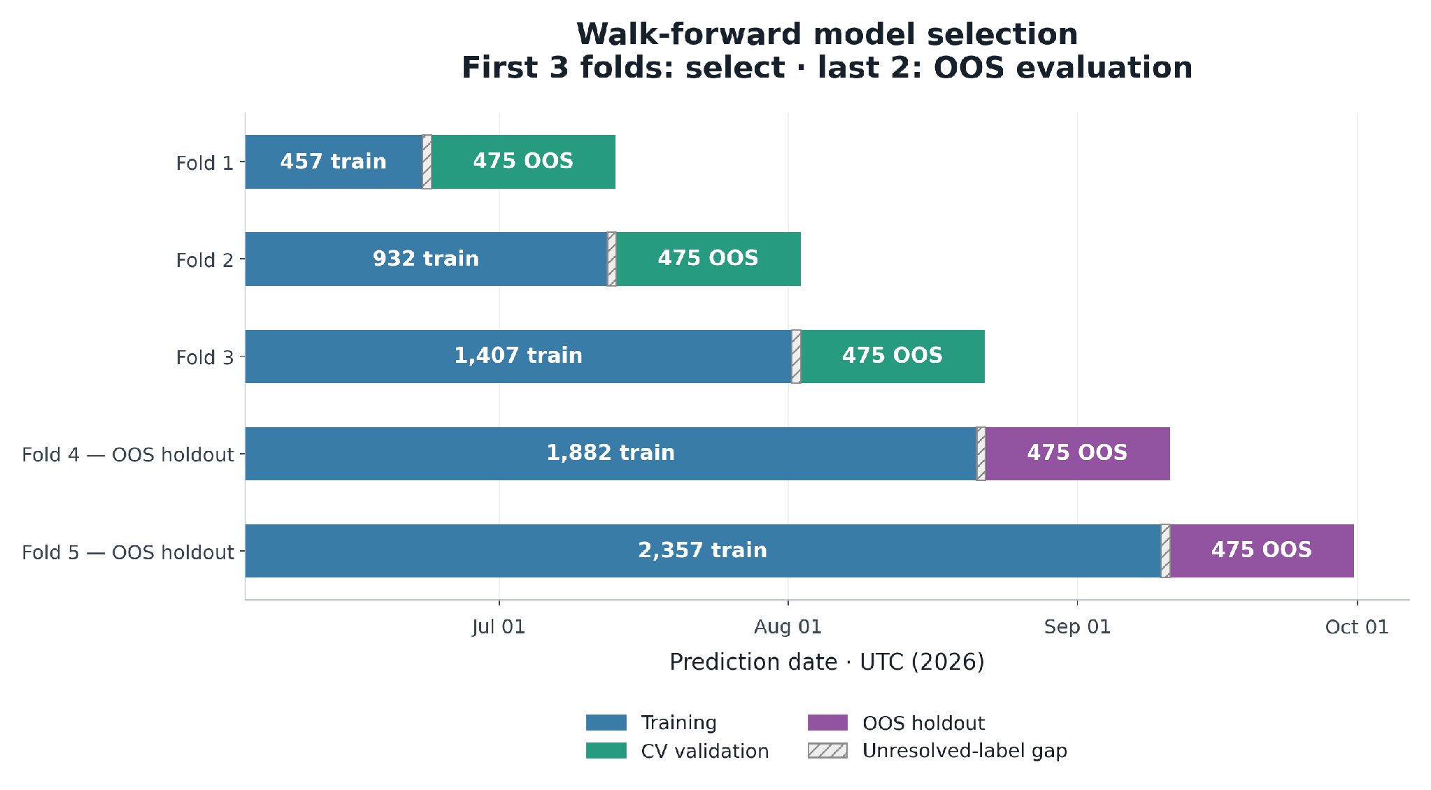
Random train/test splits are a poor fit for this example. Neighboring rows share much of their input history, and successive 24-hour targets overlap. We use expanding walk-forward folds so training always precedes evaluation.

The example script (notebooks/example_triple_barrier_walkthrough.py) exposes the model search near the top, so you can change the experiment without editing the training loop:
LGBM_SEARCH_GRID = {
'n_estimators': [25, 50, 75, 100],
'num_leaves': [7, 15, 31],
'max_depth': [3,4,5],
'learning_rate': [0.01, 0.03, 0.05],
}
# Shared settings; a parameter in the search grid overrides its fixed value.
LGBM_FIXED_PARAMS = dict(
# learning_rate=.03,
# max_depth=5,
min_child_samples=30,
random_state=42,
n_jobs=2,
verbosity=-1
)
Scikit-learn's ParameterGrid generates every combination: 4 tree counts × 3 leaf counts × 3 depths × 3 learning rates = 108 candidates. LGBM_FIXED_PARAMS applies to every candidate; a setting in the search grid overrides the corresponding fixed value.
Each candidate is evaluated on the first three folds, and the lowest mean multiclass log loss wins. Log loss evaluates the probabilities themselves: assigning high confidence to the wrong class is more costly than admitting uncertainty.
For the saved Gold run, the selected configuration was:
| Trees | Leaves | Maximum depth | Learning rate | Mean selection log loss |
|---|---|---|---|---|
| 25 | 15 | 3 | 0.03 | 1.0013 |
That configuration stays fixed for both OOS folds. The model is refitted before each fold using only labels available at its training cutoff; resolved outcomes from the earlier OOS fold can enter the later fold's training data, but never the parameter search. All performance and trading figures below combine these two folds. After evaluation, the script refits on all eligible data to create the production artifact without overwriting the OOS results.
Change the features in the same place
Immediately below the model parameters, the example exposes both a recipe list and the function that constructs features:
ENGINEERED_SPECS = [
# {'kind': 'log_return', 'window_bars': 1},
# {'kind': 'log_return', 'window_bars': 6},
# {'kind': 'log_return', 'window_bars': 24},
]
def engineer_features(frame, specs, input_bars):
"""Edit here: return (dataframe, added column names) for training AND serving.
Use only feature_* inputs, which are normalized OHLCV ratios. Compute each
row independently from its input window: serving supplies a single row.
Never use target_*/tb_* columns or shift/roll across training rows. Return
every added model feature's name. Keep imports inside this function so its
code can travel with predict.pkl; do not close over credentials/data managers.
"""
from allora_forge_builder_kit import apply_engineered_features
frame, added = apply_engineered_features(frame, specs, input_bars)
# Example custom feature (uncomment both lines to enable):
# frame['last_bar_range'] = frame[f'feature_high_{input_bars-1}'] - frame[f'feature_low_{input_bars-1}']
# added.append('last_bar_range')
return frame, added
The saved run uses the normalized OHLCV inputs with an empty ENGINEERED_SPECS list. Uncomment a log-return recipe to add it, or edit engineer_features() to implement your own transformations. The same function is captured in predict.pkl and used during live inference. Work within each row's input window: serving supplies a single row, so rolling across dataset rows would make training and inference inconsistent.
Measure the probabilities, not just the winning class
The Builder Kit's PerformanceEvaluator compares the classifier against a causal baseline made from the previous 100 resolved targets. This baseline adapts to the recent class mix without looking at future labels.
The saved run contains 950 held-out predictions, from August 22 through September 30, 2026. Worker accuracy was 53.58%, compared with 44.21% for the baseline.
| Evaluation measure | Estimate | Bootstrap lower–upper bounds | Passing rule |
|---|---|---|---|
| Accuracy improvement | +9.37 percentage points | +1.58 to +17.89 pp | Estimate > 2 pp and lower bound > 0 |
| Quadratic weighted kappa | 0.1230 | 0.0234 to 0.2166 | Lower bound > 0 |
| Brier skill | 0.2945 | 0.2463 to 0.3416 | Lower bound > 0 |
| Focal skill | 0.9390 | 0.9152 to 0.9525 | Lower bound > 0 |
| Offline coverage | 100% | — | Coverage > 90% in this offline report |
Accuracy improvement contributes two criteria, making six in total. The bounds use paired circular block bootstrap resampling: 10-row blocks, 1,000 replicates, and the 5th and 95th percentiles. Kappa accounts for the ordering of the classes, while Brier and focal skills evaluate the probability assignments relative to the baseline.
This run passed all six offline checks. That is a result for this held-out period, not evidence of live network participation: a deployed worker still needs to submit reliably. The precise criteria and formulas are in the classification evaluation reference.
Triple barrier as a distilled trading problem
The target also defines a simple trade. At each row, use the highest-probability class as a signal:
- Up: open a long position.
- Down: open a short position.
- Neutral: do nothing.
For either directional signal, exit at the first price barrier touched. If neither is touched, exit at the close of the final minute candle inside the evaluation window. The same price path that determines the label therefore determines the illustrative trade's outcome.
The walkthrough uses one unit per trade and permits overlapping positions: each hourly prediction is a separate opportunity. A long earns exit − entry; a short earns entry − exit. Barrier exits are marked at the exact boundary price, and this run uses zero transaction costs. These are simulated, target-based fills, not an execution simulation with spread, slippage, or a capital constraint.
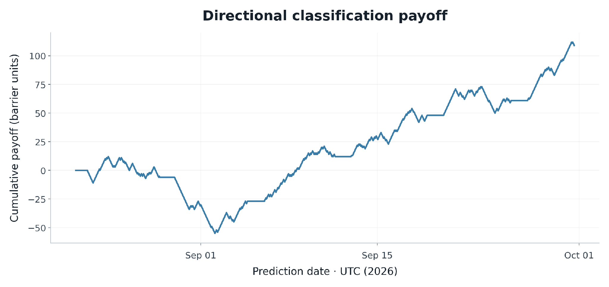
Before calculating dollar PnL, we can simplify the trade to a classification payoff. A correct directional prediction earns +1, the opposite direction earns −1, and any combination involving neutral earns zero. A declared cost can be subtracted whenever the prediction is directional; here that diagnostic cost is zero.

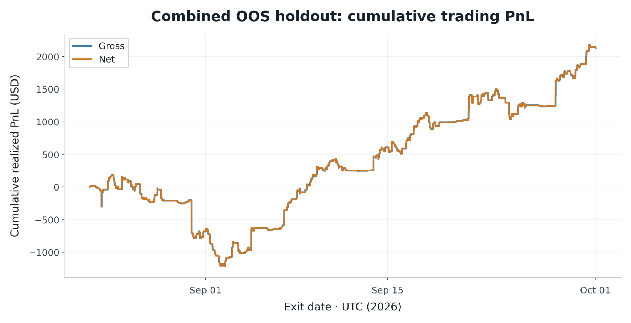
Now compare that curve with the trade ledger's cumulative realized PnL:

Both curves summarize the same directional decisions, with +109 net directional wins and positive simulated dollar PnL over this window. That connection is useful. The directional diagnostic captures much of the economic structure of the target without needing a full trading simulator.
The curves are not identical. Dollar barrier widths change between predictions, neutral expirations can earn or lose money, and the payoff chart orders observations by prediction time while the PnL chart realizes gains and losses at exit time. The dollar curve is cumulative trade PnL, not a percentage return on a fixed-capital portfolio.
Reading the confusion matrix as trade outcomes
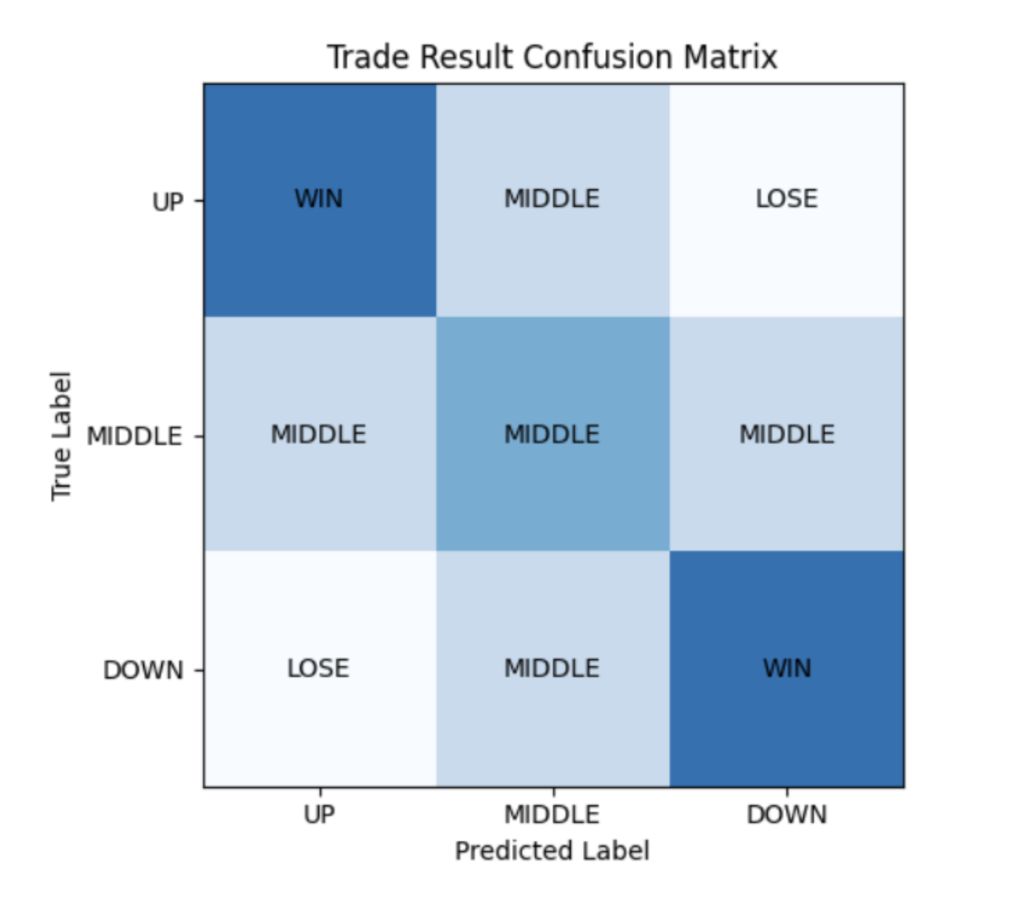
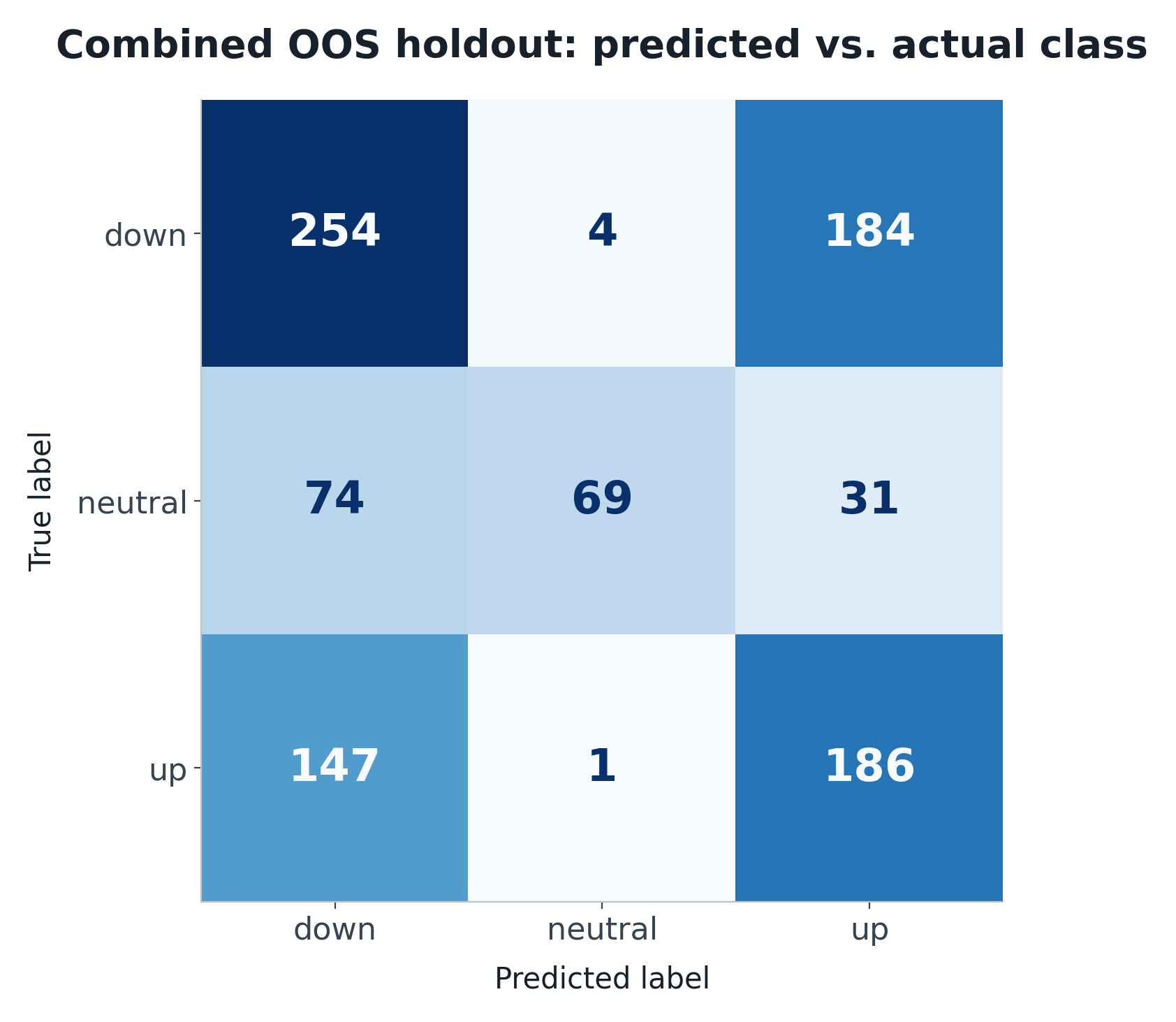
A confusion matrix makes the connection especially clear. Rows show the realized label and columns show the predicted label. Correct directional predictions occupy the top-left and bottom-right corners: these are winning barrier trades. The opposite corners are losing barrier trades.

Here is the corresponding count matrix from our held-out predictions:

The middle row and column explain why classification accuracy and trading payoff are different. Predicting neutral avoids a trade; a directional prediction followed by a neutral outcome still opens a trade, but expires without touching either price barrier. Those cases receive zero in the simplified diagnostic, while the actual expiry price determines their simulated PnL.
This gives builders a way to inspect the model beyond a single accuracy figure. Does it frequently confuse up with down? Does it avoid opportunities by predicting neutral? Are the errors concentrated in a particular market period? The example saves the underlying predictions and trade ledger so you can investigate those questions.
Run the example and start submitting
The walkthrough script produces the plots above, evaluation reports, CSV files, and a reloadable predict.pkl. Start from a clone of the Builder Kit, with an Allora API key saved locally in .allora_api_key:
python3.11 -m venv notebooks/.venv
source notebooks/.venv/bin/activate
pip install -e ".[dev]"
export REPO_ROOT="$PWD"
export ALLORA_API_KEY="$(cat .allora_api_key)"
export ALLORA_NETWORK=testnet
python notebooks/example_triple_barrier_walkthrough.py --topic 87
The outputs appear in notebooks/triple_barrier_example_output/. Run deployment from its own worker directory so the new worker has separate local state:
mkdir -p "$REPO_ROOT/notebooks/triple_barrier_example_output/worker"
cd "$REPO_ROOT/notebooks/triple_barrier_example_output/worker"
TOPIC_ID=87 \
PREDICT_PKL="$REPO_ROOT/notebooks/triple_barrier_example_output/predict.pkl" \
python "$REPO_ROOT/notebooks/deploy_worker.py"
python -m allora_forge_builder_kit.web_dashboard
WorkerManager handles wallet creation, testnet funding, registration, and the worker process. The deployment command prints the worker's log path. Follow that file with tail -f worker_logs/worker_87_<address>.log to watch registration, polling for a prediction opportunity, and submission.
Here is a real worker-log excerpt from a Gold testnet run, from wallet initialization through its first successful submission. Your address, nonce, timestamps, and transaction hash will differ:
2026-10-02 18:39:39,977 INF Worker wallet: allo1te94sw035et96phpz0872tvk00wyjt3wcqu96v || Balance: 0.000000000000000000 ALLO
2026-10-02 18:39:40,076 INF Requesting ALLO from testnet faucet...
2026-10-02 18:39:40,761 INF Request sent...
2026-10-02 18:39:45,866 INF Balance: 0.000001000000000000 ALLO
2026-10-02 18:40:02,742 INF ✅ Registered inferer allo1te94sw035et96phpz0872tvk00wyjt3wcqu96v for topic 87
2026-10-02 18:40:02,746 INF 🔄 Starting polling worker
2026-10-02 18:40:02,940 INF Topic 87: unfulfilled nonces: {11126818}
2026-10-02 18:40:02,941 INF Our unfulfilled nonces: {11126818}
2026-10-02 18:40:03,310 INF 👉 Found new nonce 11126818 for topic 87, submitting... account_seq=2
2026-10-02 18:40:27,246 INF ✅ Successfully submitted: topic=87 nonce=11126818
2026-10-02 18:40:27,246 INF - Transaction hash: CBD79794799BE3AEA449CD1367B6A5310CA7D70C68CD671C83E9C94A8921AB2A
2026-10-02 18:40:27,246 INF - View on explorer: https://testnet.explorer.allora.network/explorer/transactions/CBD79794799BE3AEA449CD1367B6A5310CA7D70C68CD671C83E9C94A8921AB2A
The worker receives a nonce, computes its labeled probability prediction using fresh Atlas data, and submits it to the network. The success line and transaction hash show the completed submission; the explorer link opens its transaction details. Open the dashboard at http://localhost:8787 to inspect submission history and the labeled values. This demonstration worker was stopped after confirmation.
To explore Silver or WTI, change both the walkthrough's --topic and deployment's TOPIC_ID to 88 or 89. To develop a different model, keep the target and labeled-probability contract, then experiment with features, estimators, and model selection. The Builder Kit supplies the working path from historical observations to a live worker; the topic documentation defines the prediction task that every model shares.
Explore the topics on Allora Forge
Visit each testnet topic on Allora Forge to explore the prediction task and participating models:
- Gold — topic 87: forge.allora.network/topics/87?network=testnet
- Silver — topic 88: forge.allora.network/topics/88?network=testnet
- WTI oil — topic 89: forge.allora.network/topics/89?network=testnet